VRE droughts matter more for prices than reliability
Long duration VRE droughts are not that long or that severe. Nevertheless electricity spot prices are very elastic so we need to distinguish between the implications of droughts for reliability and the implication for prices.
The analysis below leads me to think that 24 hour continuous periods where wind and solar output was less than 66% of average will happen only about 6% of the time. That’s not a drought by the standards of rainfall. Its hardly even a dry season. Rain droughts can go for years.
This article only focusses on utility wind and solar, uses the 2035 capacities by REZ assumed in the 2024 ISP for 2035 and then applies those capacities to the ISP weather traces. On that basis…
There are fewer than 0.5% of days where wind and solar output will be below 66% of normal for four days or longer in a row.
Even on those extreme days 8 GW of dispatchable power running continuously for a week would cover the short fall as can be seen from fig 10. That’s the sort of event that open cycle gas or diesel generation can indeed cover, although even the fuel for that would probably need storage.
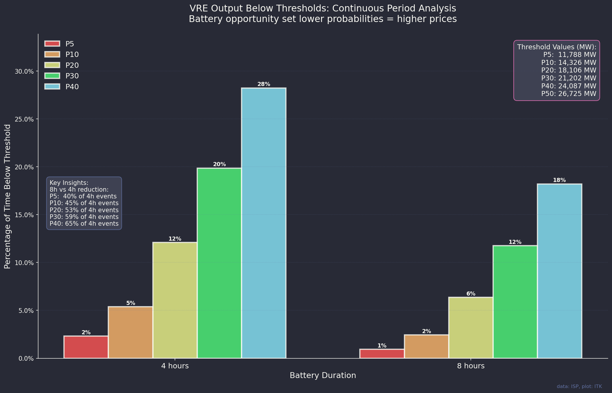
By contrast we can look at the much higher frequency of low outputs over 4 and 8 hours.
It’s not the way I normally analyse things but the following plot is one way of thinking about the relative opportunity set for four and eight hour batteries. P5 is where hourly output is in the lowest 5% of hours for either four or eight continuous hours. P40 is where output is in the lowest 40% of hours for four or eight continuous hours. It’s likely that prices will be highest for the P5 and lowest in this plot for the P40 events. So the plot gives an idea of the likely high price events. For 8 hour batteries there are far fewer opportunities to use the full 8 hours. But then 8 hour batteries have much lower unit costs than 4 hour batteries
Long duration storage is cheaper because it sacrifices power for lower cost
Storage is often divided into short, medium and long duration classes. Duration is defined as the quantity of storage/power (maximum rate) at which it can be delivered or charged.
Generally the longer the duration the storage the cheaper it is on an energy basis The cheapness comes because by definition long duration storage can only be delivered or recharged slowly. The cheapness comes because power is sacrificed for duration.
Measured on a power basis a long duration storage system is likely to be more expensive than a short duration system. At today’s price 2 GW of 4 hour batteries would cost no more than $3.2 bn compared to Snowy 2 cost of $12 bn. 2 GW of 4 hour batteries can be built and connected in 18 months. I suspect 2 GW of 8 hour batteries could be done for under $5 bn. So I’d need a lot of convincing about the value of that extra duration before I wanted to spend 4X the money and have a much lower round trip efficiency.
For pumped hydro the total cost of the storage divides between the pumping or generation power, the tunnel capacity, and the size of the dams. Dams have an economy in that volume grows at 2/3 the cube of the radius. So expanding the radius by say 2 metres adds close to 6 cubic metres of storage. In practice for pumped hydro though this advantage has to be offset against, the fact you need two dams, plus the race or tunnels needed to circulate the water up and down. There are in fact lots of other disadvantages.
\(V = \frac{1}{2} \cdot \frac{4}{3} \pi r^3 = \frac{2}{3} \pi r^3\)
For lithium batteries the total cost divides between the cost of the inverters and the cost of the cells. Each cell of a given class has the same cost as every other cell. The economy comes because you use less inverters and put the cells in parallel instead of in series.
Again the point is that to get lower cost for a given quantity you have to sacrifice power.
Data and methods
AEMO provide 12 reference years of wind and solar traces . That data set provide the output (capacity factor for each 30 minutes) for a 1 MW standardised wind turbine or solar farm for every REZ for every half hour for a 34 year forward period. That adds up to about 2.5 bn data points. Not something you want to open in Excel necessarily.
Although I could have worked with just the weather data I decided to use AEMO modelled capacities installed and so enabling the calculation of gross energy output for each of those half hours. To do that I used the wind and solar capacities that were installed as the beginning of 2035 in the 2024 ISP. AEMO provides that data. This has the advantage of being:
- practical, AEMO only installs wind or solar in some REZs ones where obviously they model to have transmission available; and
- is the capacity required, with the other generation ie rooftop, hydro, batteries, gas to keep the lights on;
- by 2035 in the central ISP scenario there is virtually no coal left.
So for each of 12 reference years, for 34 calendar years (408 sample years) of forecast with each reference year running from 2021 to 2055. Each of the 34 years of each reference year has 17520 half hours in the year. And for each of those half hours we have 34 REZs. The code takes the wind and the solar capacity in each REZ and multiplies by the capacity factor for that half hour in that REZ. Of course this doesn’t allow for physical or economic curtailment or MLFs. Actual output if this capacity was installed would be less. On the other hand rooftop solar is excluded as are all other forms of generation. Its just about utility wind and solar.
General results and profile
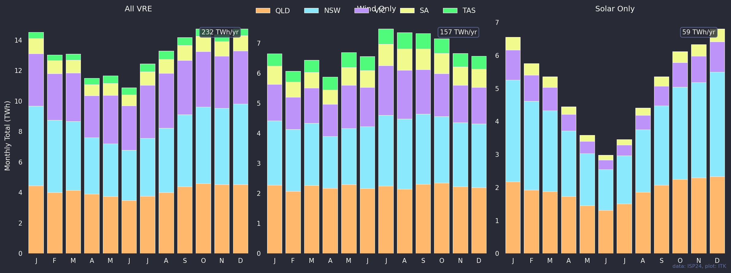
There are lots of visualisations in this section. Let’s start with how the wind and solar capacity is installed by State in 2035 in the 2024 ISP Central Scenario. It’s this one set of capacities that are used in all other plots. Perhaps the most obvious point is how much is installed in QLD. That’s what Queenslanders are currently cutting off their noses to spite their faces for. A chance to be leader.
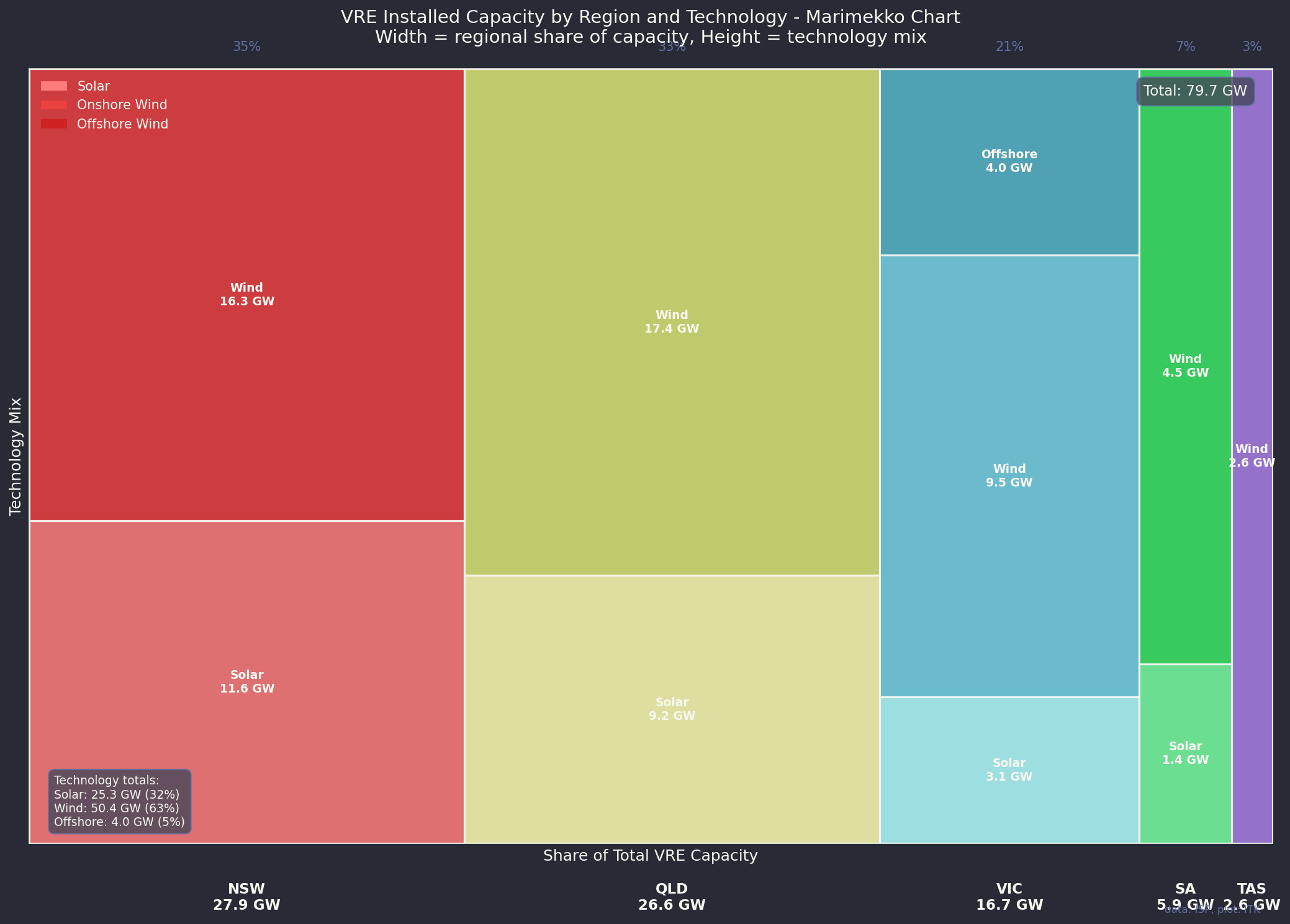
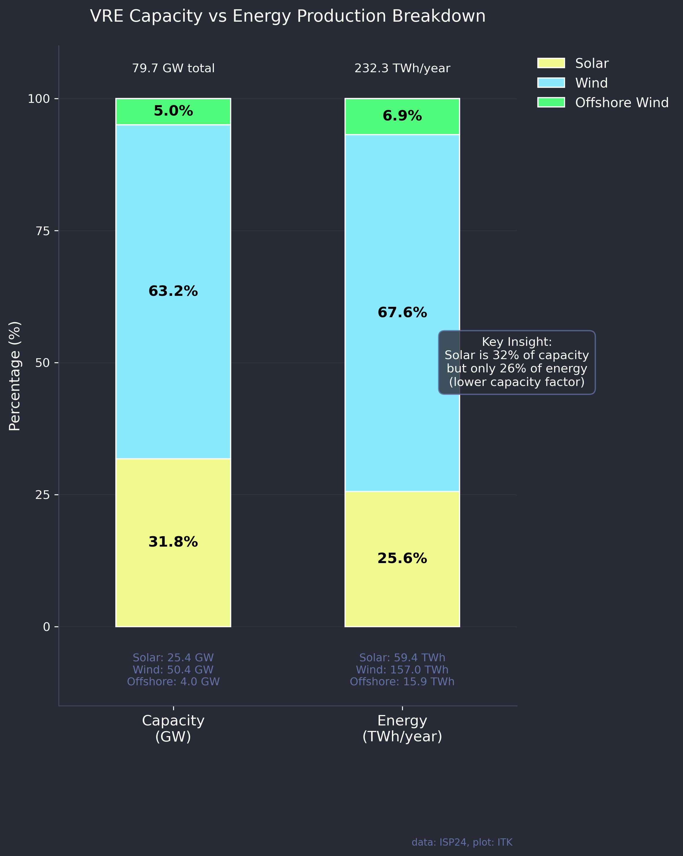
So the 2024 ISP was dominated by wind but also included, because it’s Victorian Govt policy, some offshore wind. And because capacity factors of solar are less than wind, about 70% of the utility scale VRE is wind.
And then this is the output expressed as an index over the year also showing the P5 and the P95 lines. P5 means that 5% of observations are less than that line, P95 that 95% of observations are less than the line. The data was smoothed a bit to make the message such as it is more obvious.

And we can look at the average day which will have a very familiar shape.
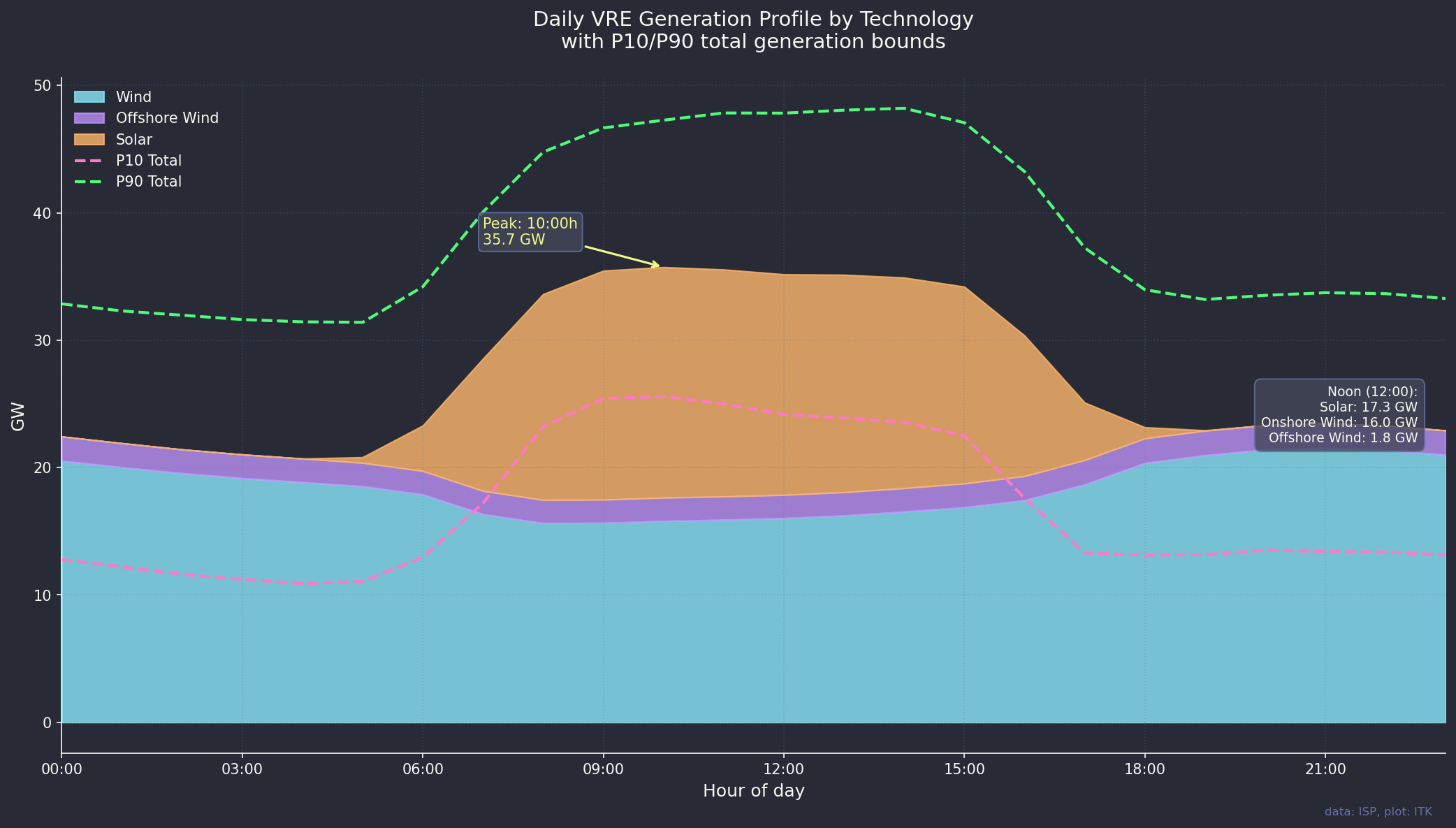
The output is actually relatively steady month to month and that’s because QLD provides a very steady baseline. Wind is the middle plot of the three. Again note that all these plots exclude rooftop.
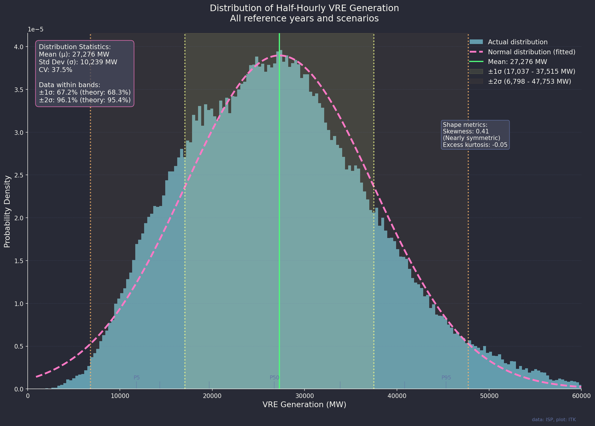
Finally in this general section we can look at the distribution of output and it is close enough for jazz as a normal distribution
Variability and droughts
Compared to rainfall there are no droughts. Rain droughts can go on for years. The sun shines every day. We can rearrange the output to show percentiles of daily, weekly and monthly averages. Just like P5 and P95 these plots show the percentage of days or weeks where the output is less than the xth percentile.
I’ve shown this chart as an index, P50 for each series is the median, not the mean.
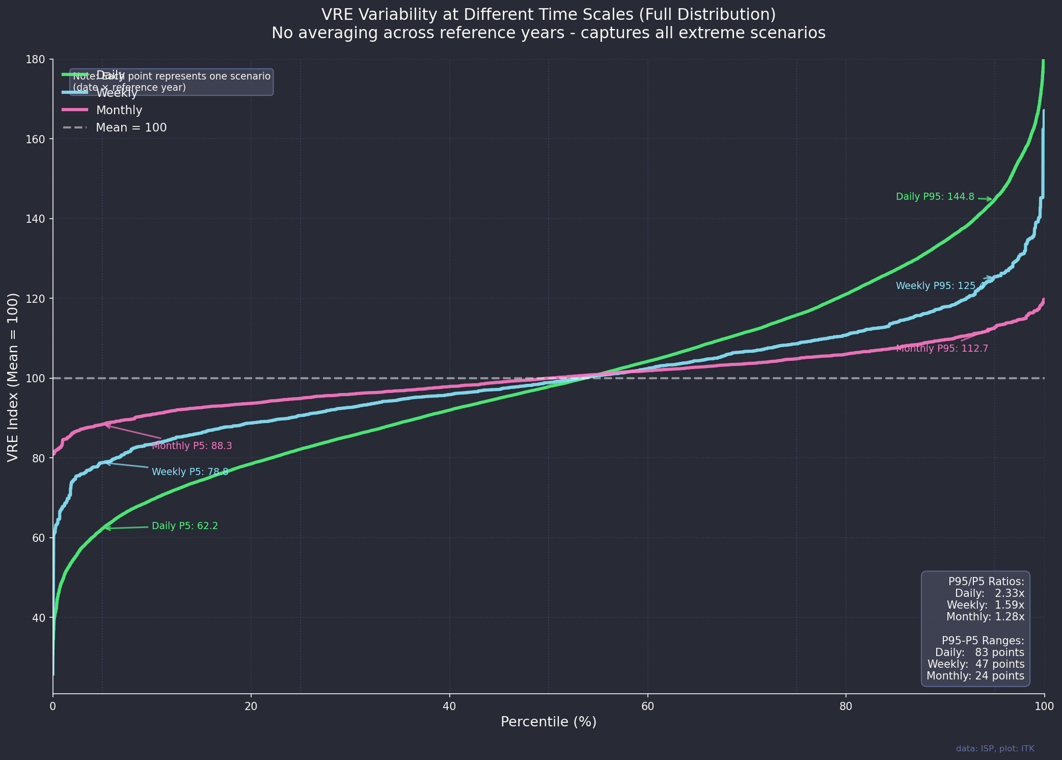
On a monthly basis there is no month where output is less than 80% of the median.
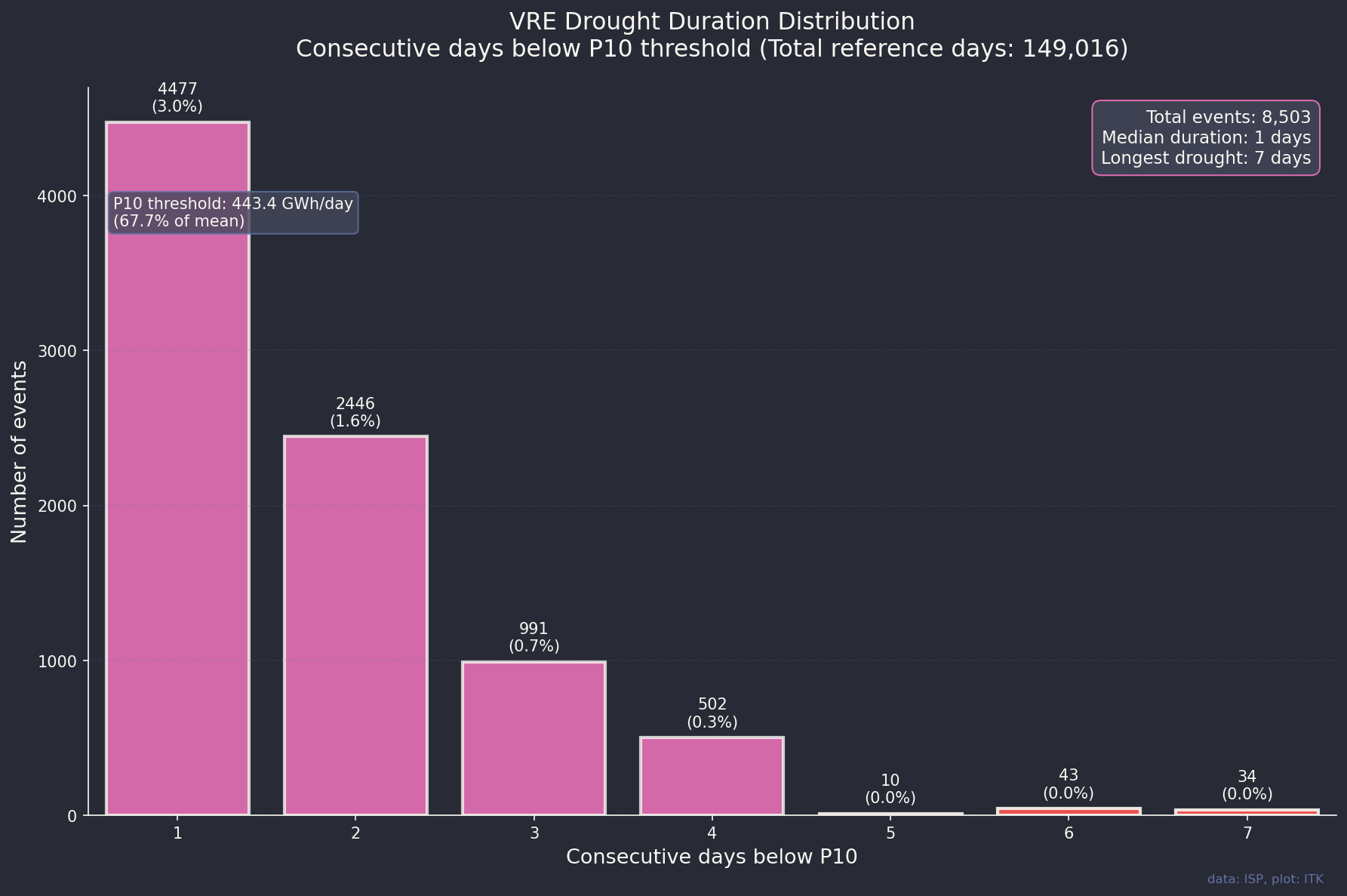
What about these famous cold Winter months we hear so much about. Well this plot captures all the sequences of a day or longer where output was in the lowest 10% of days. Note that the 10% cutoff point still has output at roughly 2/3 of average output, that is the P10 threshold output for a day is 443 GWh which about 68% of average day output. Down but far from zero. Using that threshold a drought of 4 days or longer happens about 0.5% of the time.
If we add up the output of the 4 days and longer droughts we can compare the average day of an extreme drought with the average day over the entire set.
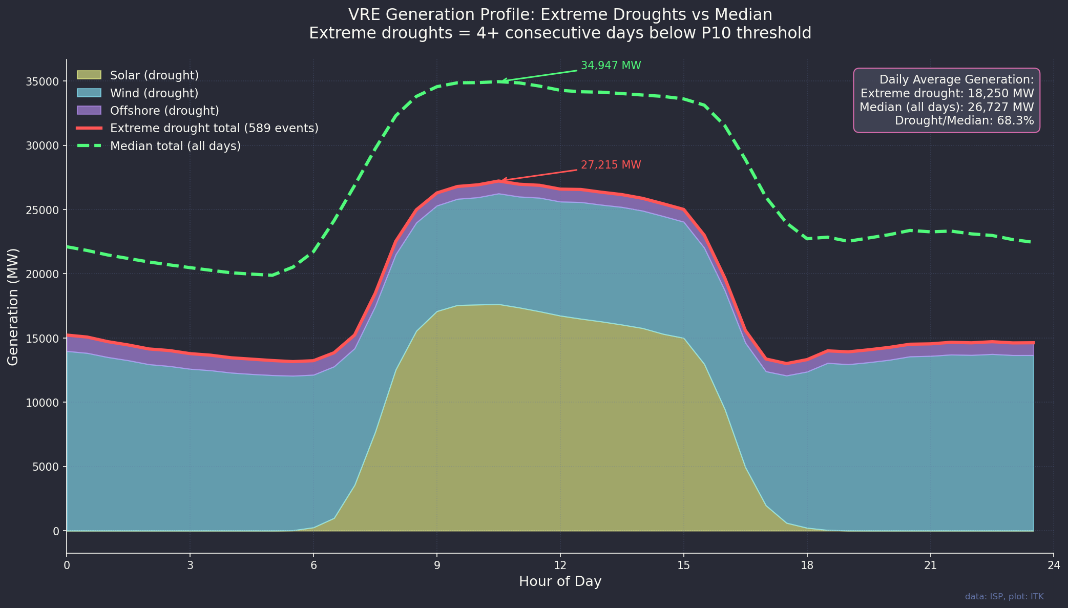
My takeaway from this last plot is that around 8 GW of reserve capacity capable of operating for a week is required. Of course its not that simple but it does provide a visible sizing dimension.
Trading and planning thoughts
June, July and August are less predictable than other months. So if you are a trader you would want to consider your downside as well as the upside.
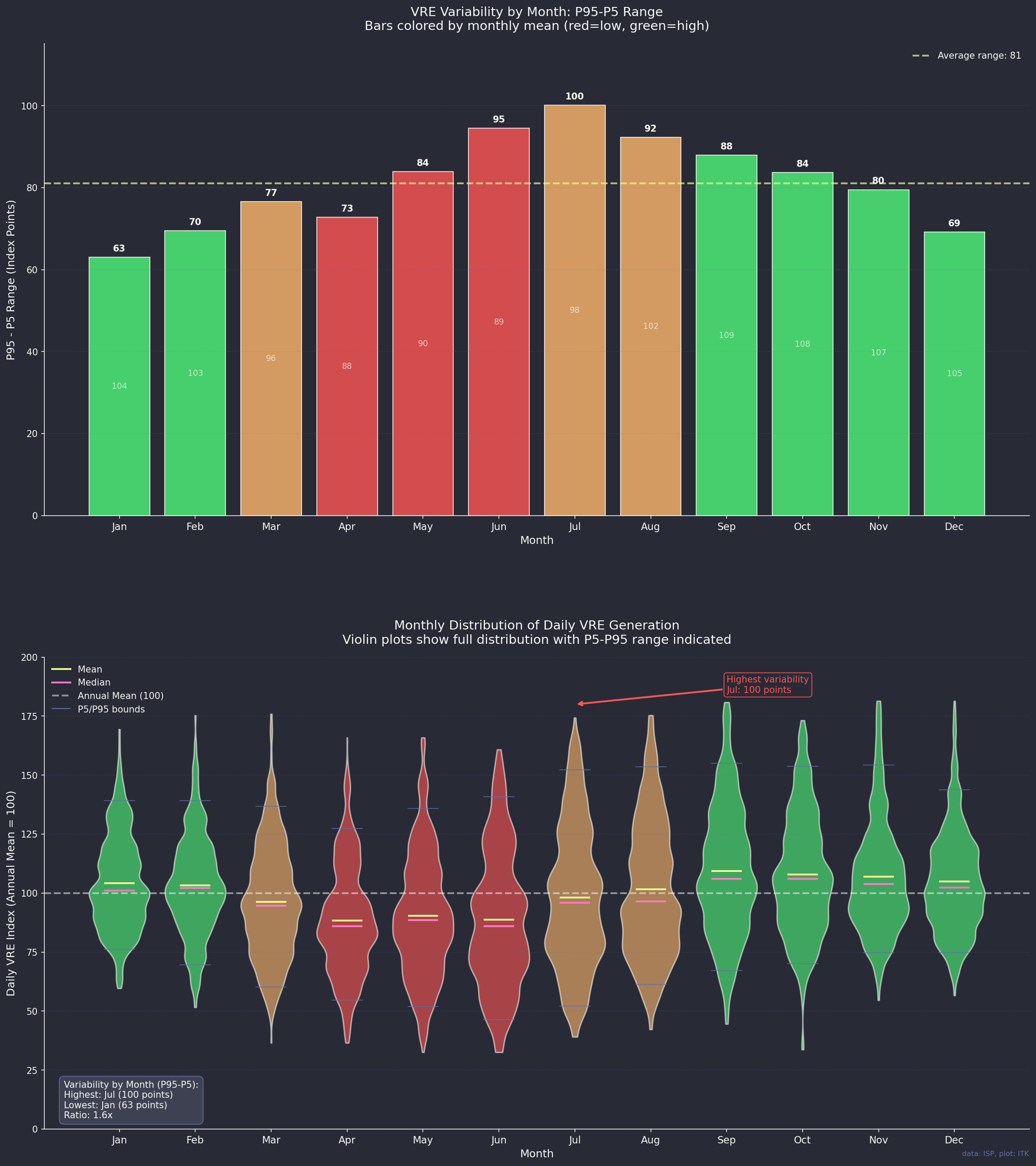
It also looks to me, and I am not a trader, that between say March and September there are more times when the number comes in below the average than there are times when it comes in above. This may mean that being short in those months will mostly prove to be a profitable strategy but stands the risk of being completely wrong.
Supplement: How meteorologists define droughts
Threshold-Based (Percent-of-Normal)
A simple and commonly used definition involves comparing observed precipitation to a long-term average. A drought occurs when precipitation falls below a defined percentage of that average over a specific period.
- Example: Precipitation is less than 75% of the 30-year mean over a 3-month period.
- The percentage threshold and timescale may vary by region or application.
Duration-Based
A drought is often defined as lasting a minimum time period, such as several weeks or months.
- Example: No significant rainfall for at least 14 consecutive days.
SPI (Standardized Precipitation Index)
- Based purely on precipitation data.
- Converts rainfall into a standardized normal distribution.
- Can be calculated over 1-, 3-, 6-, 12-month periods to capture short- and long-term droughts.
Classification:
- SPI < -1.0 → Moderate drought
- SPI < -1.5 → Severe drought
- SPI < -2.0 → Extreme drought
Rainfall Deficit (Anomaly)
A simple but effective method is to look at the rainfall deficit:
Deficit = Mean rainfall - Actual rainfallThis method helps estimate cumulative shortfall over a defined time period.
Whether for rainfall, wind, or solar, you can define a drought using several key attributes:
| Attribute | Example Description |
|---|---|
| Threshold | Rainfall < 75% of long-term average |
| Duration | At least 2 continuous weeks |
| Severity | SPI < -1.5 or large cumulative deficit |
| Frequency | Number of droughts per season or year |
| Recovery | Time taken to return to average or normal levels |