1. The basic idea: weather as an initial-value problem
A weather forecast is a physics calculation. The atmosphere is a fluid on a rotating sphere, heated unevenly by the sun. Its behaviour is governed by a set of equations — conservation of momentum, mass and energy, the gas law, and the thermodynamics of water changing phase — that have been known since the 19th century.
In principle, then, forecasting is simple:
- Measure the state of the atmosphere everywhere, right now.
- Solve the equations forward in time.
Both steps are much harder than they sound, and the reasons shape everything about how forecasting is done.
Step 1 is hard because you can never measure everywhere. The atmosphere is continuous; observations are scattered points. Whatever you don’t measure, you have to estimate.
Step 2 is hard because the equations can’t be solved exactly. You have to chop the atmosphere into a three-dimensional grid of boxes and step forward in small time increments, which introduces approximation error at every step. And because the system is chaotic, small errors don’t stay small.
The chaos point is the fundamental one. In the early 1960s, meteorologist Edward Lorenz found that tiny differences in the starting conditions of a simple atmospheric model produced completely different outcomes within a modest amount of simulated time. This is the “butterfly effect”, and it isn’t a limitation of our computers — it’s a property of the atmosphere itself. Even with perfect equations and near-perfect observations, useful deterministic weather forecasts run out somewhere around 10 to 15 days. Beyond that, you can still say useful things, but they’re statements about the statistics of the weather, not about specific days.
That single fact is why forecasting splits into distinct timescales, each with its own methods. We’ll come back to that in Section 7.
2. Step one: observing the atmosphere
Every forecast starts with data. Modern systems ingest millions of individual observations for each model run, drawn from a wide range of instruments.
Surface Automatic weather stations measure temperature, humidity, wind, pressure and rainfall at fixed points. Rain gauges and river gauges feed flood models. These are dense in populated areas and sparse everywhere else.
Upper air Weather balloons carrying radiosondes are launched — typically twice daily — and transmit temperature, humidity, pressure and wind as they ascend to around 25–30 km. Australia launches from about 38 sites, including the Antarctic Territory. Balloons remain the gold-standard vertical profile, but they’re expensive and there are only about 1,000 launch sites worldwide.
Radar Weather radar emits microwave pulses and measures what bounces back off raindrops, hail and snow. Reflectivity gives rainfall intensity; the Doppler shift gives the wind velocity along the beam. Dual-polarisation radars (which transmit both horizontally and vertically polarised pulses) can distinguish rain from hail from melting snow by the shape of the particles. Australia’s network mixes 1980s–2010 “legacy” units, a locally designed “Wurrung” upgrade deployed from 2017, and newer dual-polarisation radars from European manufacturers deployed from 2019.
Satellites This is the single biggest data source globally — roughly 90% of the observations that go into a modern global model come from space. Two types matter:
- Geostationary satellites sit 36,000 km above a fixed point on the equator and image the same hemisphere every 10 minutes or so. Japan’s Himawari series covers the Australian region.
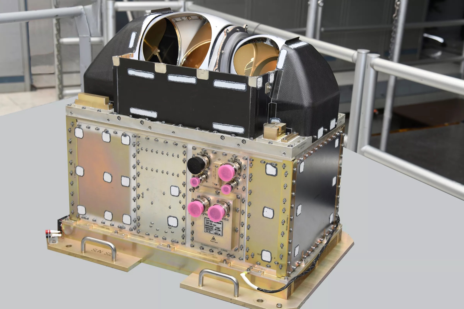
- Polar-orbiting satellites fly at ~800 km, circling pole-to-pole roughly every 100 minutes while the Earth rotates beneath them, building global coverage twice a day. These carry the microwave sounders that measure temperature and humidity through cloud — the most valuable satellite data for forecasting.
Aircraft Commercial aircraft report temperature, wind and pressure automatically along their routes, providing dense upper-air data over flight corridors — and almost none over the oceans and the empty interior.
Ocean Drifting and moored buoys, tsunami-detection (“tsunameter”) buoys on the sea floor, tide gauges, ship-based instruments, and Argo floats — autonomous devices that drift at depth, surface every ten days to transmit a temperature and salinity profile, then sink again. Ocean data barely affects tomorrow’s forecast; it drives next season’s.
The Australian difference: an observational disadvantage
Australia sits downwind of some of the emptiest ocean on Earth. Weather systems arriving in Perth or Adelaide have crossed thousands of kilometres of Indian and Southern Ocean containing almost no surface stations, no radiosonde sites, and few aircraft flights. Northern-hemisphere forecast centres, by contrast, have dense observing networks upstream of most of their populated areas.
This has three consequences:
- Satellite data matters more here than almost anywhere. Australia relies heavily on satellite radiances to constrain the initial state over the oceans. This is why the Bureau of Meteorology invests research effort in squeezing more out of each satellite instrument — including recent work on assimilating Chinese FY-3E microwave sounders and GPM satellite radiances.
- Australia has no meteorological satellite of its own. It operates ground reception stations but depends entirely on the satellites of international partners — Japan, the US, Europe, China. The Bureau published a “mission requirements document” for an Australian microwave sounding instrument in late 2025, which signals live interest in changing this.
- Free international data exchange is not optional for Australia. The World Meteorological Organization framework under which countries share observations without charge is what makes forecasting here possible at all.
3. Step two: data assimilation — turning observations into a starting state
You now have millions of observations, scattered irregularly in space and time, of varying quality, measuring different things. The model needs something quite different: a single value for temperature, humidity, wind and pressure in every box of a global three-dimensional grid — tens of millions of numbers. Most boxes contain no observation at all.
The process of getting from one to the other is called data assimilation, and it is the most sophisticated part of the whole enterprise.
You don’t start from nothing. You start from the previous forecast. A six-hour forecast from six hours ago is already a good estimate of the current state — it’s called the “background” or “first guess”. Data assimilation then adjusts that background to be more consistent with the new observations, weighting each by how much you trust it against how much you trust the model.
The leading method, 4D-Var (four-dimensional variational assimilation), does this by treating it as an optimisation problem: find the atmospheric state that, when run forward through the model, best fits all the observations collected over a time window, while staying close to the background. “Four-dimensional” means observations are used at the actual time they were taken, not lumped together. This requires running the model backwards as well as forwards: assimilation often consumes as much computer time as the forecast itself.
The output is called the analysis: the best available estimate of the atmosphere right now. It’s then used both to start the forecast and as the background for the next cycle, six hours later. The system runs continuously, forever.
Australia’s global system upgraded to APS4 with a technique called En4DEnVar, which blends variational assimilation with information from an ensemble about how errors are distributed on any given day.
A byproduct: if you re-run this whole process over past decades with a fixed modern system, you get a reanalysis — a physically consistent gridded history of the atmosphere. Australia’s regional versions are called BARRA. These are the backbone of wind and solar resource assessment, because they give you consistent hourly weather at any location for 40+ years, which observations alone never could.
4. Step three: the model
Grids, timesteps and resolution
The model divides the atmosphere into a grid — horizontally into boxes, vertically into layers — and steps forward in time. Australia’s global model, ACCESS-G, uses boxes of roughly 12 km in the mid-latitudes and 17 km in the tropics, with 70 vertical levels. ECMWF’s global model, generally regarded as the world’s best, runs at about 9 km with 137 levels.
Halving the grid spacing costs roughly 8–16 times more computing, because you have more boxes in two horizontal dimensions and you must also shorten the timestep for numerical stability. This is why forecast centres are among the largest supercomputer operators in the world, and why resolution improves slowly.
Parameterisation
Anything smaller than a grid box can’t be simulated directly, but much of it matters — individual clouds, turbulence, the drag of hills, radiation absorption, plant transpiration. These are handled by parameterisations: sub-models that estimate the aggregate effect of small-scale processes from the large-scale variables the model does resolve.
Parameterisation is where most model error lives, and where most model development effort goes. Convection is the hardest case. A thunderstorm is a few kilometres across, so a 12 km global model cannot represent one; it has to guess how much convective rainfall a grid box produces from its temperature and humidity profile. These schemes are imperfect, and convective rainfall is the single largest source of forecast error in the tropics and in Australian summer storms.
Convection-permitting models
The way around this is to shrink the grid until storms are explicitly resolved — roughly 1–4 km. At that scale you switch the convection parameterisation off and let the model build storms itself. These models can’t run globally (too expensive), so they run over limited regions, taking their boundary conditions from the global model.
Australia runs ACCESS-C at about 1.5 km over separate domains around Sydney, Melbourne/Tasmania, Brisbane, Perth, Adelaide, Darwin and north Queensland, plus a ~2 km city ensemble. Everything between the cities gets a coarser forecast, which for a continent this empty is a gap. The Bureau’s response has been ACCESS-A, a pan-Australian convective-scale model developed through 2025 to replace the patchwork of city domains with continuous coverage.
These models produce far more realistic storm structure — squall lines, sea breezes, orographic rainfall — but they don’t necessarily put the storm in the right place. The gain is in realism of character, not accuracy of location.
Coupling
Modern systems increasingly run the atmosphere coupled to an ocean model, a wave model, a sea-ice model and a land-surface model, exchanging heat, moisture and momentum at each timestep. Australia runs OceanMAPS for the ocean and AUSWAVE (built on WAVEWATCH III) for waves. For short forecasts, coupling is a refinement. For seasonal forecasts, it’s the whole game.
5. Step four: ensembles — forecasting the uncertainty
Because of chaos, a single forecast is a single draw from a distribution of possible outcomes. Running one and presenting it as the answer discards the most useful information available: how confident should you be?
The solution is the ensemble. Run the model many times from slightly different starting conditions — perturbations within the range of observational uncertainty — and, in modern systems, with slightly different model physics too. Where the members agree, confidence is high. Where they diverge rapidly, it’s low.
Ensemble spread is not noise; it is the forecast of the forecast’s own reliability, and it varies from day to day. A stable high-pressure system might produce members that agree for a week. A cut-off low near the NSW coast might produce members that diverge within 48 hours.
Ensembles are also what makes probabilistic forecasting possible. “70% chance of rain” comes from something like: 35 of 50 members produced rain at that location. Australia’s global ensemble, ACCESS-GE, runs at about 33 km — coarser than the deterministic model, because you’re paying for many runs instead of one. That tradeoff between resolution and ensemble size is one of the central design decisions in operational forecasting.
6. Step five: post-processing and the human forecaster
Raw model output is not a forecast. A grid box represents an area average at a nominal height; a weather station is a specific point in specific terrain. Models have systematic biases — too warm overnight in valleys, too windy in sheltered places, drizzle where there should be none.
Statistical post-processing corrects this by comparing years of past forecasts against what actually happened, and learning the corrections. Techniques range from simple bias correction to machine-learning methods. Australia’s operational system is called IMPROVER, developed jointly with the UK Met Office. This stage also calibrates probabilities: if the raw ensemble says 70% and it only rains 50% of the time when it says that, the system fixes it.
Human forecasters remain in the loop, but their role has shifted. They rarely draw the forecast now; they adjudicate between models, apply local knowledge, judge whether a system is behaving as the model expects, and make warning decisions, where the cost of a miss and the cost of a false alarm are asymmetric and the judgement is as much social as meteorological.
Verification closes the loop. Every forecast is scored against what happened, using metrics chosen for the question: root-mean-square error for temperature, Brier score or CRPS for probabilistic forecasts, and specialised measures for rainfall, where getting the pattern nearly right shouldn’t be scored the same as getting it completely wrong. Verification is how you know whether an upgrade helped.
7. The timescales
This is where the different pieces of machinery separate out. Each timescale exploits a different source of predictability.
Nowcasting: 0 to 6 hours
Too short for the model chain to help much — by the time a global model has assimilated, run and been post-processed, the next few hours are already underway. Nowcasting instead works directly from observations, chiefly radar extrapolation: track where the rain is and how it’s moving, and project it forward, with statistical rules for how cells grow and decay. Australia’s system is called STEPS, and blends radar extrapolation with NWP as lead time increases. Satellite imagery, lightning detection and surface observations supplement it. This is the domain of flash flood and severe thunderstorm warnings.
Short range: 1 to 3 days
The sweet spot for convection-permitting regional models. This is where forecasts are most useful and most accurate: daily maxima and minima, rainfall, wind, fire weather, frost. A modern three-day forecast is about as good as a two-day forecast was two decades ago.
Medium range: 3 to 10 (or 15) days
Global models and their ensembles. Regional models add little here because errors flow in from the boundaries. Skill degrades steadily with lead time, and the useful product shifts from specific values to probabilities and pattern guidance. Beyond about day 10, deterministic skill is largely gone.
Sub-seasonal: 2 to 6 weeks
The awkward middle. Too far out for initial conditions to carry information, too near for slow ocean signals to dominate. It was long called the “predictability desert”. Skill comes from slowly evolving phenomena that modulate the odds of weather without determining specific days:
- the Madden–Julian Oscillation (MJO), a pulse of tropical convection that circles the globe every 30–60 days and strongly influences northern Australian rainfall and monsoon bursts;
- the Southern Annular Mode (SAM), which shifts the westerly storm belt north or south and is a major control on southern Australian rainfall and wind;
- stratospheric events, which can propagate downward and lock in surface patterns for weeks.
This timescale has improved over the last decade and matters increasingly to energy and agriculture.
Seasonal: 1 to 6 months
Here predictability comes almost entirely from the ocean, which holds far more heat than the atmosphere and turns over far more slowly — sea surface temperature anomalies persist for months, and they bias atmospheric circulation for as long as they last. Seasonal forecasting therefore requires a coupled model: atmosphere, ocean, land and ice run together.
Australia’s is ACCESS-S2, developed with the UK Met Office, running the atmosphere at about 60 km — deliberately coarse, because you need to run a very large ensemble for a very long time. Real-time outlooks use 99 members. The output isn’t “it will rain on the 14th”, it’s “there’s a 70% chance of above-median rainfall this season”.
The drivers Australia cares about are distinctive:
- ENSO — El Niño/La Niña in the Pacific, the single strongest influence on Australian rainfall variability;
- the Indian Ocean Dipole (IOD), which matters more for Australia than for most countries and drives much of the winter–spring rainfall signal in the south-east;
- SAM, again, on longer timescales.
Northern-hemisphere centres are heavily focused on ENSO and the North Atlantic Oscillation; the IOD is comparatively an Australian and Indian Ocean rim preoccupation. Seasonal systems are calibrated against hindcasts — the model re-run over 30+ past years — which is the only way to know what its probabilities mean.
Decadal to climate projection: years to a century
At this range you are no longer forecasting weather at all. Initial conditions are irrelevant; what matters is the boundary conditions — greenhouse gas concentrations, aerosols, land use. Climate models answer a different question: given emissions scenario X, what does the statistical distribution of weather look like in the 2050s?
These are projections, not predictions. They are run as scenario ensembles across many international modelling centres (coordinated through CMIP), and downscaled to regional resolution for national use. Australia’s downscaling systems are BARPA (and a convection-permitting version, BARPA-C), which take coarse global projections and dynamically refine them over the Australian region — necessary because a 100 km global climate model cannot see the Great Dividing Range.
8. The AI disruption
Since about 2022, machine-learning weather models have gone from curiosity to operational reality.
The approach is different. Rather than solving physics equations, these models are neural networks trained on decades of reanalysis data to learn the mapping from the atmospheric state now to the state six hours from now, then applied repeatedly. Google DeepMind’s GraphCast and Huawei’s Pangu-Weather were the first demonstrations; ECMWF built its own, the AIFS, and made the deterministic version operational in February 2025 and the ensemble version in July 2025, with a version 2 upgrade in May 2026.
The advantages:
- Speed. A ten-day global forecast runs in minutes on a handful of GPUs, versus hours on a supercomputer. That’s roughly three orders of magnitude less energy.
- Skill. On standard verification scores, these models now match or beat physics-based models for many variables and lead times.
The caveats:
- They are trained on reanalysis, which is itself produced by physics models and data assimilation — so AI forecasts currently depend on the conventional system continuing to exist.
- Models trained to minimise average error tend to produce smooth, blurry fields, under-representing extremes — which is what matters most for warnings.
- They have no explicit physics, so they can violate conservation laws and there’s no guarantee they’ll behave sensibly in a climate state outside their training data.
The near-term picture is hybrid rather than replacement: AI for cheap, fast, large ensembles; physics for the assimilation, the extremes, and the coupled ocean.
Australia has not tried to build a rival global AI model. The Bureau has focused instead on making the technology useful locally: calibrating ECMWF’s AI forecasts for Australian conditions using a technique called RainForests, and verifying machine-learning against physical models for high-stakes cases like tropical cyclone rainfall. For a mid-sized agency with limited compute, adapting and evaluating is the affordable strategy.
9. Australia versus the world: a summary
| Dimension | Global leaders (ECMWF, NOAA, Met Office) | Australia |
|---|---|---|
| Global model resolution | ~9 km (ECMWF) | ~12 km (ACCESS-G) |
| Model lineage | Independently developed | Built on the UK Met Office Unified Model, via a long-standing partnership |
| Satellites | Own fleets (US, EU, Japan, China) | No sovereign meteorological satellite; reception stations only |
| Observing density | Dense upstream networks | Very sparse upstream (Indian, Southern Ocean) |
| Compute | Tens to hundreds of petaflops | ~4 petaflops (Australis II, a Cray XC50/CS500 delivered 2020) |
| Key seasonal drivers | ENSO, NAO, Atlantic SSTs | ENSO, IOD, SAM, MJO |
| Distinctive hazards | Winter storms, hurricanes, tornado outbreaks | Bushfire weather, tropical cyclones, east coast lows, monsoon, flash flooding |
The overall picture: Australia contributes more to the science than its size would suggest, but operates at a structural disadvantage in observations and computing. Its strategy has been collaboration — shared model development with the UK, free data exchange under the WMO, reliance on partner satellites — plus focused investment where local conditions differ from the northern hemisphere and imported science doesn’t transfer: fire weather, tropical cyclones, the monsoon, and the rainfall dynamics of the Australian south-east.
10. What to remember
- A forecast is a probability distribution, not a number. The ensemble spread is information, not a caveat.
- The 10–15 day limit is physics, not engineering. No amount of computing will make a specific-day forecast for three weeks out.
- Different timescales use entirely different sources of predictability — initial conditions for days, tropical convection and the stratosphere for weeks, ocean heat for months, radiative forcing for decades.
- Much of the improvement over the last 40 years came from data assimilation and better observations, not from faster computers alone.
- Forecast skill has improved by roughly one day per decade for the last several decades. The skill ECMWF achieved at three days in 1980 now extends to about six days.
Key sources
- Bureau of Meteorology, ACCESS NWP data information (APS4 model configurations and resolutions): https://www.bom.gov.au/nwp/doc/access/NWPData.shtml
- Bureau of Meteorology, ACCESS-S climate forecast system: https://www.bom.gov.au/government-and-industry/research-and-development/research-and-development-projects/access-s-climate-forecast-system
- Bureau of Meteorology, Bureau Research Report series index (recent research directions): https://www.bom.gov.au/government-and-industry/research-and-development/research-publications
- Australian National Audit Office, Bureau of Meteorology’s Management of Assets in its Observing Network, Auditor-General Report No. 21 2024–25 (observing network structure): https://www.anao.gov.au/work/performance-audit/bureau-of-meteorologys-management-of-assets-its-observing-network
- ECMWF, AIFS machine learning data and implementation notes: https://www.ecmwf.int/en/forecasts/dataset/aifs-machine-learning-data