A coal free NEM @ $107/MWh still wants 50 GW of wind
TL;DR
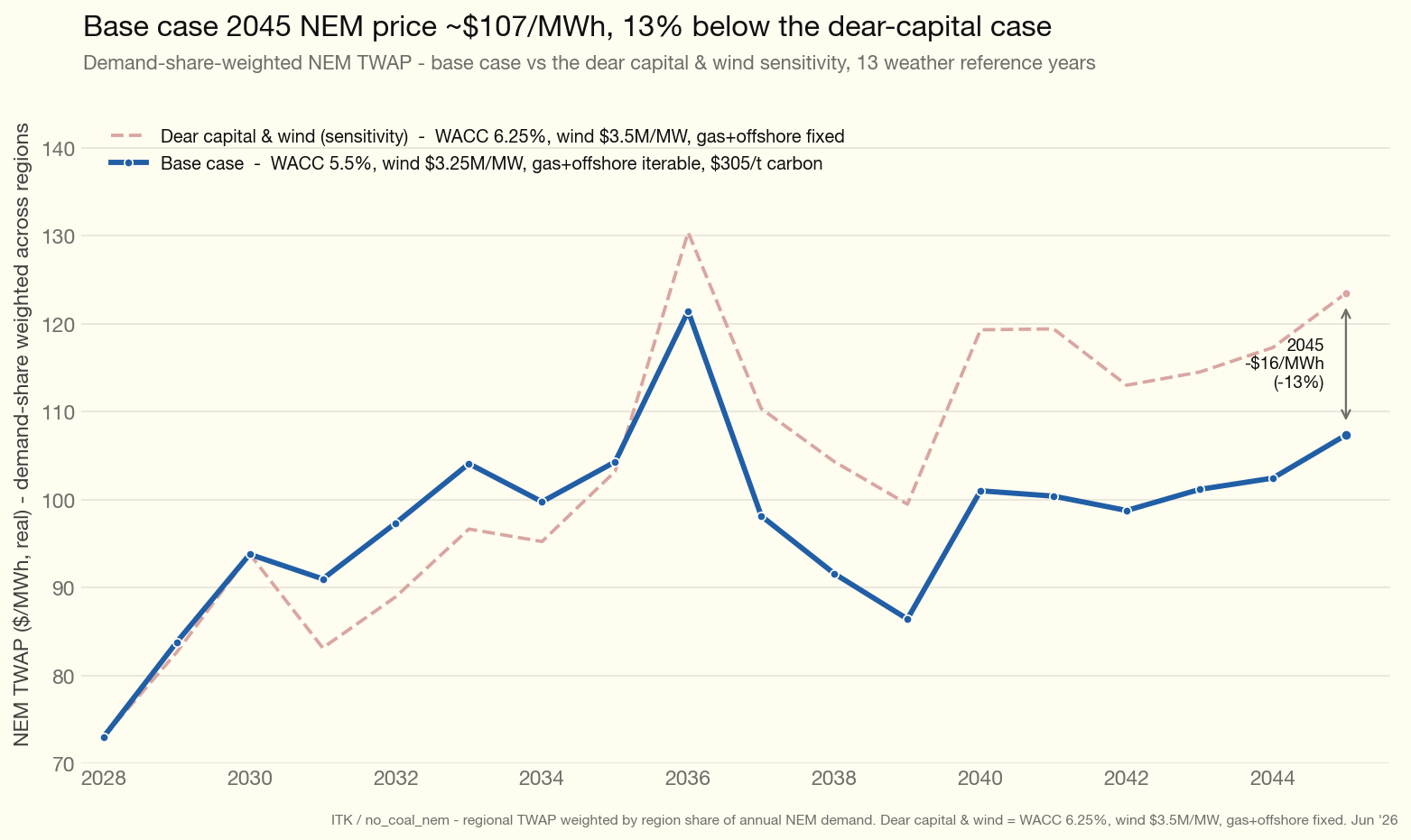
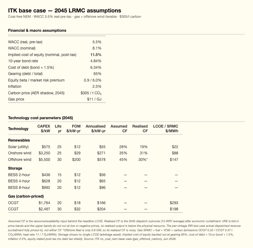
My estimate of the spot price for electricity in a coal free NEM in 2045 is about $107/MWh. That price assumes onshore wind costs $3.25 m/MW in real terms and that in 2045 there is a carbon price of $305/t in line with the AER carbon cost trajectory. The 2045 LRMC calculation used a 5.5% real pretax WACC which equates to a nominal return on equity of 11.5%.
Even using $3.5 m/MW cost of wind right through to 2045 a system that achieves LRMC in 2045 (my chosen end point) has about 50 GW of wind. This is a key outcome of the modelling. Even with wind at much higher cost than assumed in GenCost the best outcome for consumers is when we build plenty of onshore wind.
I ran simulations with Victoria’s offshore wind target fixed and others where the outcome was determined by the LRMC, using a 2045 offshore wind capex of $5.5 m/MW. In the base case scenario just 1 GW of offshore wind was built. In practice that won’t happen. The LRMC process, as I could have predicted, substitutes cheaper onshore wind in Tasmania for offshore Bass Strait wind, and also builds more gas.
Once a 2045 coal free capacity mix was set and with a more or less known 2028 starting portfolio a trajectory was built from start to finish. The process starts with a linear build path but is then modified to ensure that plant built in each year (vintage) earns WACC over its lifetime. In the end about 76% of all region/year/technologies earned lifetime WACC.
Despite including a steep carbon cost the 2045 LRMC portfolio does have some gas. If you leave the carbon cost out, more combined cycle gas is built with fewer batteries and less open-cycle gas. Also of note all of this modelling assumes QLD stays open 5 years longer than assumed in the ISP. Even so the modelling makes clear that consumers are better off if the replacement capacity is built early.
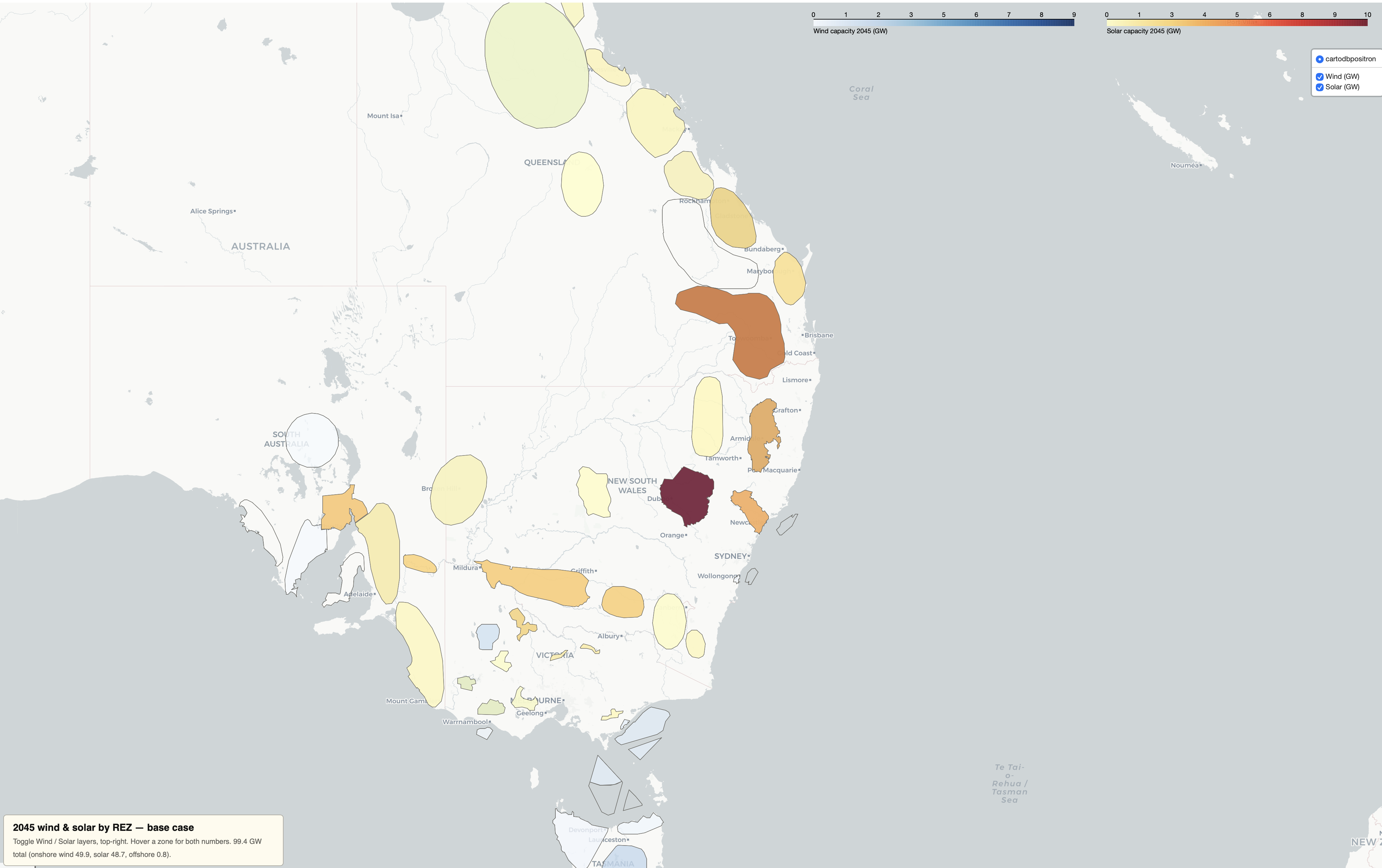
As explained later the LRMC process works out which region to build capacity in to make sure everything earns a return and consumer prices are managed. Within a region capacity is allocated to REZs in the same proportion as the ISP does.
Process, tools and the role of the ISP
At the core of the process is Vertex, ITK’s dispatch model of the NEM built by consultant to ITK, Paul Bandarian over a two year period. Given a fleet of capacities and a year of half-hourly conditions — wind and solar capacity factors at the REZ level (from AEMO’s weather traces), regional demand, fuel and carbon prices, transmission limits, and the coal/gas/hydro fleet — it solves a linear program that co-optimises generation and storage across time and returns the marginal (shadow) price in each region for every half hour. It does this for every year from 2028 to 2050, across 13 historical weather years (2011–2023), with the fleet updated each year — about 25 million half-hourly regional prices per run. Storage charging and discharging are decided by the model, not assumed; scarcity prices emerge from demand-response and value-of-lost-load tiers when supply is tight. The headline price I quote is a time-weighted average of each region’s half-hourly prices, then averaged across regions weighted by each region’s share of NEM demand.
Available capacity is divided into 162 bid bands plus some buy bands for storage — assumptions about how much capacity each generator (or storage unit, on both its charge and discharge sides) offers at each price. These allocations are judgement calls, calibrated against historical bidding patterns and adjusted for how behaviour is expected to change (for instance as coal exits). They are the model’s main calibration lever: because the half-hourly price is set by the marginal band’s bid, the bands are what let the model reproduce realistic market prices rather than pure marginal cost.
The capacity forecast is developed in three steps: a 2045 end point, a 2028 starting point, and then a build trajectory between them.
One of the key insights from the process is a view of what a post coal operational NEM fleet might look like. To do this we used a standard LRMC process. That is we took assumptions about capex, WACC and operating capacity for each fuel technology and then ran a linear program that dispatched the fleet in 2045, looked at the returns each technology earned and then adjusted the fleet size until each technology was approximately earning WACC.
In the base case the fleet ends up with 50 GW of wind, 49 GW of solar and 45 GW of batteries, plus about 10 GW of gas. Plenty of building to do yet. (The high-cost-of-capital sensitivity, by contrast, builds 62 GW of batteries and only 7 GW of gas: with carbon-priced gas in the mix, cheaper combined-cycle gas displaces some medium-duration battery storage.)
Demand
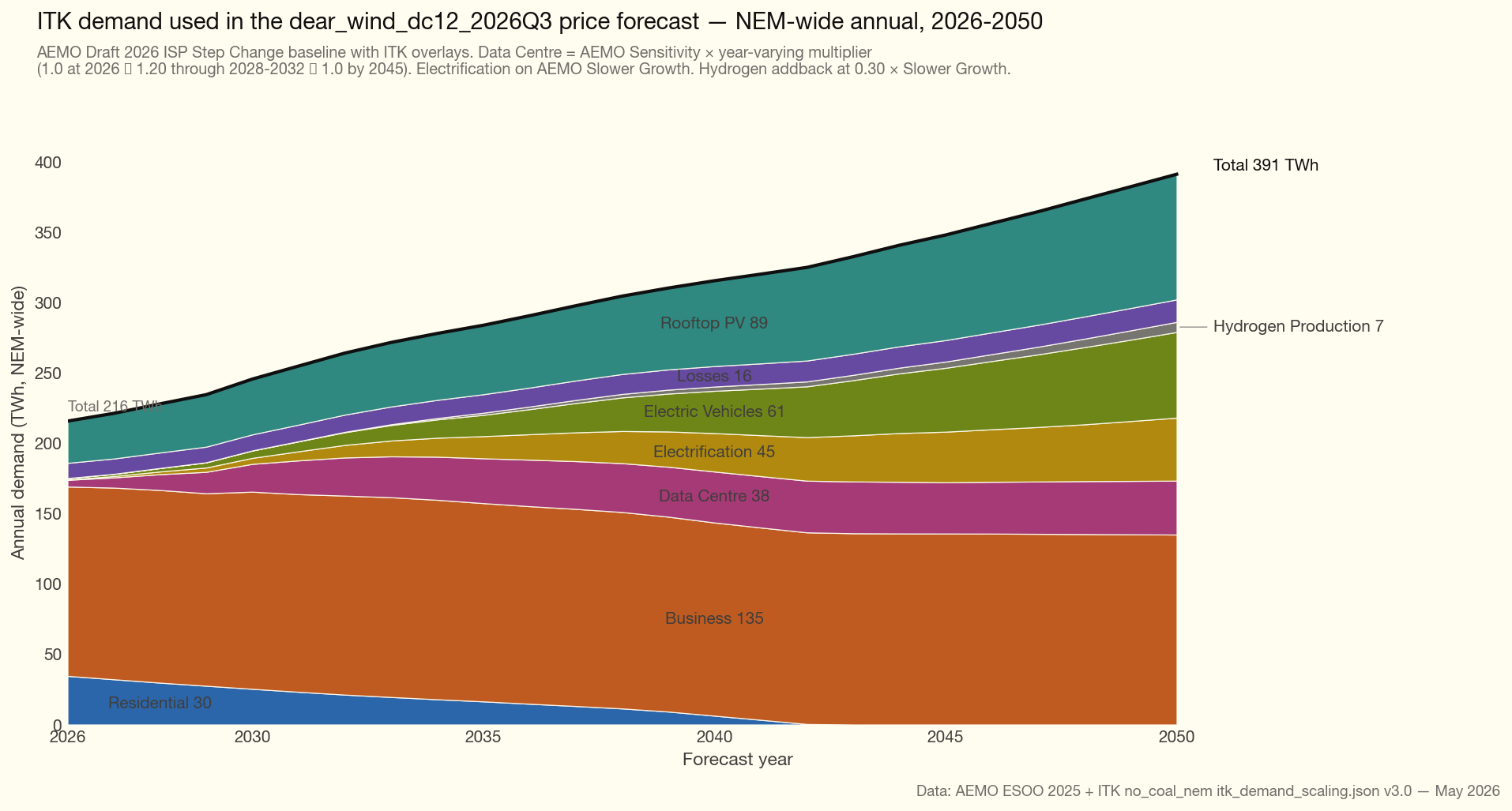
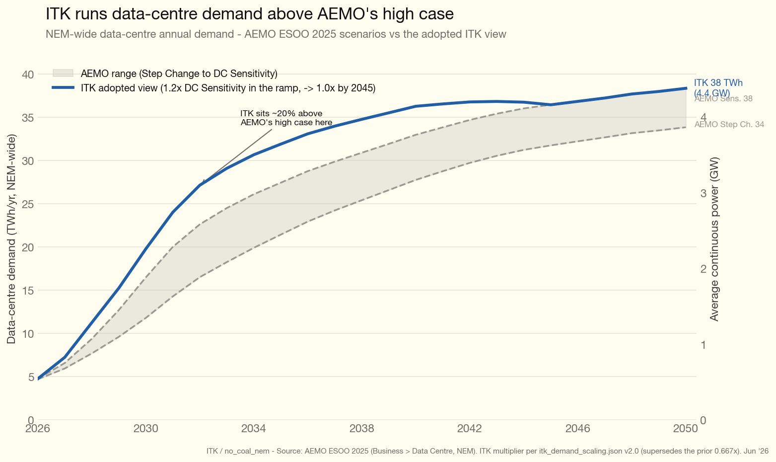
I started with AEMO’s ISP P50 demand traces. Then sharply reduced the out year hydrogen, modestly reduced electrification and in the end increased data centre demand in the early years with a convex curve so that by 2050 it ends up in the same place. A point that emerged during the study was the higher the data centre demand, the higher the firming required, because the it flatterns the load: a high-load-factor data centre runs through the night and through low-wind, low-solar periods, so it pulls firm capacity at exactly the hours solar cannot serve. My own view — not a direct model output — is that data centres will need to bring their own firming, and that this will benefit the system.
Data centres - volume and uptime requirement
Behind the meter batteries, fast then slower
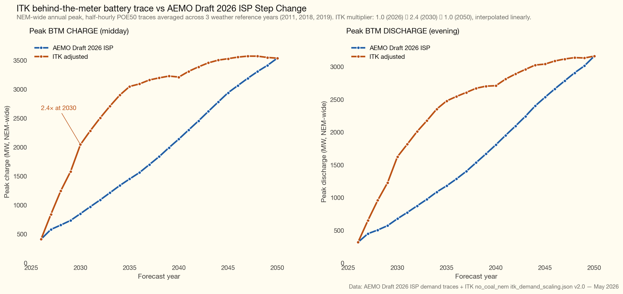
In this modelling BTM batteries and solar are an input. I “adjusted” AEMO’s “OPSO” series for our BTM batteries and rooftop numbers. You can see the difference between AEMO and ITK’s behind the meter battery supply. I project recent growth which is at a faster rate than AEMO. So these numbers reflect the Bowen home battery plan outcomes but end up at the same point as AEMO projects. I preserved AEMO’s daily shape of charge and discharge.
Capacity costs - High wind capex is assumed
The ISP central case and the range of 2045 capex assumptions that I used for sensitivity testing is shown in the following plot. Also shown are the base case values chosen.
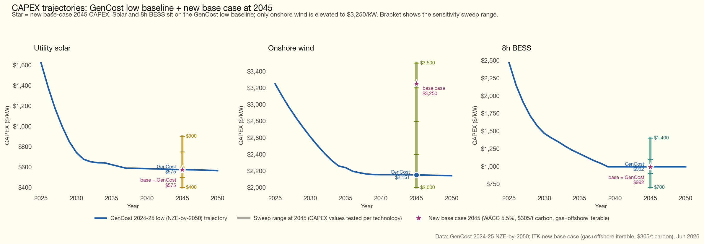
You can see that I tested a range of wind capex much above that assumed for the GenCost Central case.
A plot that shows the sensitivity of the LRMC optimised capacity in 2045 for various wind, solar and battery costs is shown below. This particular plot had offshore wind and some gas as fixed inputs and the results may vary slightly if all technologies had been iterated.
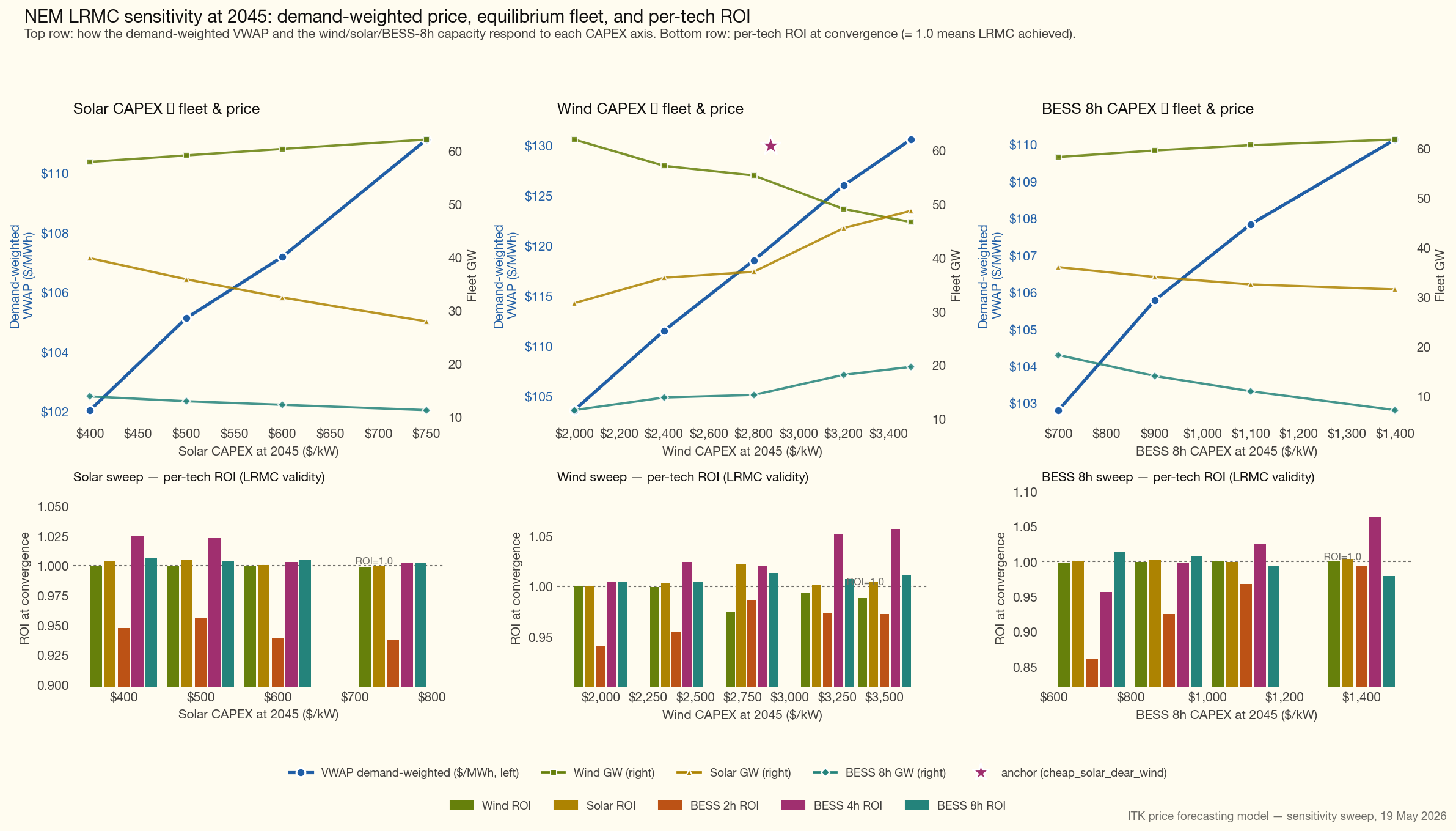
The key points I take from the plot are:
- VWAP is more sensitive to the wind capex assumption than it is to the solar or battery capex cost.
- But that sensitivity is relative. Even at high wind capex the LRMC still has plenty of wind in the capacity mix.
- Battery capex is less important than the quantity of battery storage. That the batteries exist is what matters, not so much what they cost.
Building the capacity trajectory
We start from a 2028 capacity floor — the committed projects in AEMO’s Committed Development Project list (CDP4) — and a fixed 2045 endpoint, the long-run-marginal-cost (LRMC) equilibrium fleet in which each technology earns its cost of capital in that single year.
Between the two fixed endpoints we build a year-by-year trajectory. The starting shape is a convex front-load for solar and BESS.
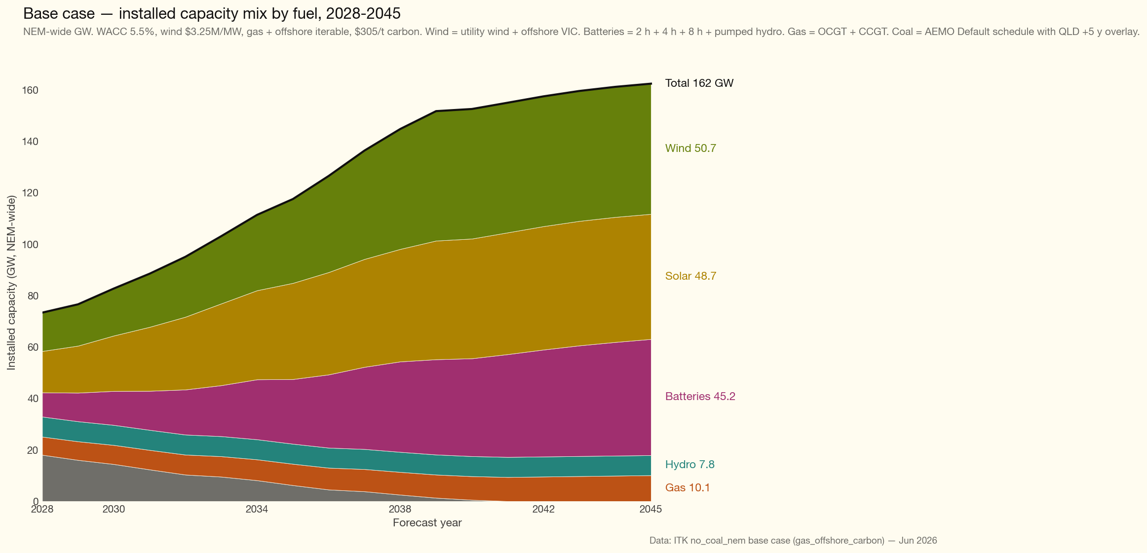
The build follows a front-loaded curve: capacity goes in fastest in the early years and tapers off as 2045 approaches. Concretely, by the mid-point of the 2028–2045 period (around 2036) about three-quarters of the new solar and battery capacity is already built, with the remaining quarter added over the back half.
Wind was held to a perhaps optimistic build-rate cap of 3.5 GW/year NEM-wide (solar 4, BESS 3 GW/year each).
The front-loading is deliberate. As Queensland coal retires — and it may retire faster than replacement capacity can be built — under-building in those years would let prices spike. Bringing the replacement forward avoids that. The bottom line: even if Queensland insists on running its coal generators for longer, consumers are still better off when the replacement capacity is built earlier.
A single-year 2045 equilibrium, however, does not guarantee that a unit built earlier recovers its cost over its lifetime: early vintages pay higher (earlier) capex on a falling cost curve and earn through the low-price transition years. So I test the trajectory against a vintage-WACC criterion — every unit of each technology, in every build-year and region, must earn at least its WACC over its asset life, valued at the prices the trajectory itself produces across 13 weather reference years. I measured this with a full-surface audit that computes a lifetime IRR for every (technology, region, build-year) increment.
I then re-shape the trajectory to clear that hurdle by deferral. Because the 2028 floor and the 2045 endpoint are both fixed, there is no net change to capacity — instead the build is either deferred or accelerated. Build that is failing its lifetime return is deferred out of the early, low-price years into the later 2030s and early 2040s when prices have recovered, conserving the total build and respecting the build-rate caps. Each iteration targets the worst-returning technology-and-region. In the base case a deferral round lifts the share of investible vintages from about 74% to 76%; the remainder is structurally hard to fix — capacity locked into the 2028 floor that cannot be moved, early-2030s storage that earns below its hurdle at low transition-year prices, and Queensland VRE held down by the interconnector.
Note that for each iteration the technologies were dispatched across all weather years and over the horizon of 2028 to beyond 2050 and for 17,520 half hours. If you think about it that’s a lot of sums.
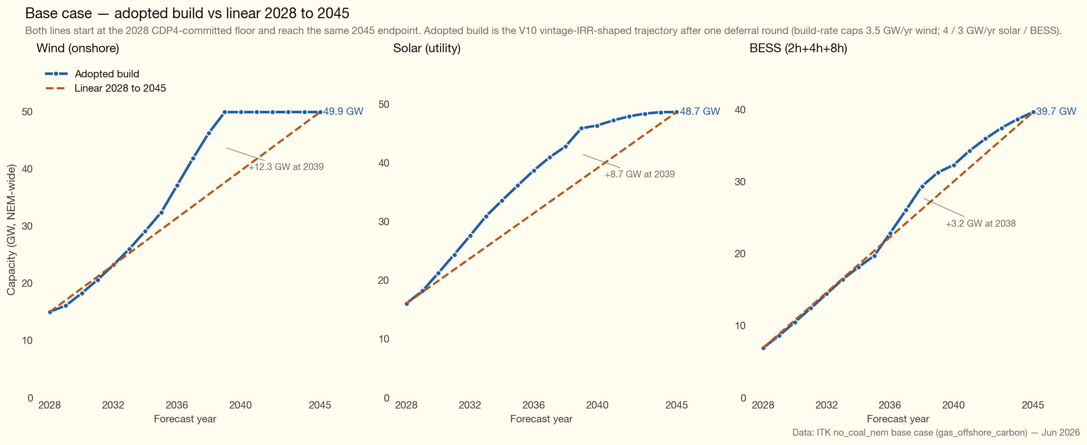
AEMO’s ISP has also typically ended up building wind before solar although for all I know the reasons might be quite different.
Capacity is allocated to regions by the LRMC equilibrium (each region iterated to earn its cost of capital, then reshaped by the vintage-IRR step). The REZ capacity factors don’t drive this allocation directly — the model inherits AEMO’s REZ build-stack as the spatial template and only applies the half-hourly capacity-factor traces afterward to convert each zone’s allocated MW into generation; the zone-level resource quality therefore enters only implicitly, via AEMO’s own tendency to weight its build-stack toward higher-yield REZs.
The process has a soft penalty that tries to keep time weighted prices in a region in any year below $110/MWh. As you can see that threshold is still breached around 2036 — a mid-2030s winter scarcity peak that shows up in every version of the model, base case and sensitivities alike, as Queensland coal exits faster than firm replacement arrives. It is not caused by the high capex or high cost of capital. However it’s possible that with more optimisation lower TWAPs could be achieved. But i get bored.
Nor does every vintage of each technology actually earn its lifetime cost of capital. In a couple of construction years solar earns below WACC on a lifetime basis. And some vintages of batteries also struggle. In fact when I brought the optimisation process to a halt 4 hour and 8 hour batteries were competing against each other and the sculpting process hadn’t yet found an optimal solution.
Assumptions
The table shows both an assumed and a realised capacity factor for wind and solar. The assumed figure (wind 35%, solar 28%) is the physical resource that sets the headline LCOE; the realised figure (wind 31%, solar 19%) is what the dispatch actually produces after economic curtailment. VRE is bid in price bands and the upper bands do not run at low or negative prices, so realised output sits below physical availability — solar takes the bigger haircut because it generates into its own midday glut. The vintage-IRR test values each unit on its actual dispatched revenue, so this curtailment is priced into the returns, not assumed away.
In conclusion - I did it my way (with AEMO’s help)
I did this work because I have been trying to prove — to myself first and anyone who would listen second, for a decade or so — that Australia could have a globally competitive electricity price in a no-coal world.
Although I think the Vertex model has been developed to a professional standard and the 2045 LRMC calculation stands on firm foundations I nevertheless have come to realise that (1) no one is interested in the long term outlook for electricity prices. If they were there would be lots more literature on the topic (2) I don’t have the academic background to be taken all that seriously.
When forecasts are required it’s generally more important to the client who the forecaster is rather than understanding how the numbers were produced.
And that’s ok. In the very end I produced these numbers for my own benefit. When I get on my soapbox and talk about the impact that data centres will have, or the impact of closing coal, or building more transmission etc etc I have my own modelling tools developed to what I believe is at least a semi academic standard that I can rely on. I don’t need to quote BNEF or EY or Baringa or even Aurora. That’s not to say I won’t read and learn from everyone else, but I have my own independent numbers. Having blown the trumpet I must also acknowledge the work is only possible with the leg-up that AEMO provides on weather year capacity factors and half hourly demand time series. I just get to play with the ingredients and make my own soufflé.
Not only that but the process requires long hours of assumption checking. When developers buy forecasts from professional firms there may be large teams of people, checking transmission build dates, keeping home battery forecasts up to date, inputting data centre demand, keeping an eye on technology build costs, revisiting bid band data and so on. I get to do all that myself with no external verification, no checking, just do the work and publish. And ultimately that is not quite the professional standard. But as I say, I’m up for coffee.
Much, much more detail is available if there is a reason to discuss methodologies, assumptions or conclusions.